/K5DVT/Projects/Voltage Drop

Voltage Drop

Voltage drop calculation is essential in electrical engineering to ensure that electrical devices receive the correct voltage. This write up focuses on calculating voltage drops in lighting circuits.

Forward

Voltage drop calculations were one of the major roadblocks in early 20th century. Ohm's law was derived by Georg Ohm in 1827, so the affects of lighting's high current demands were mathematically obvious. By the Late 1800s with widespread electrification and the light becoming a staple of the home, the industry (and insurance adjusters) adopted installation codes later to be known as the NEC (National Electrical Code). Electrical shocks and fires were the primary concern and are still as every bit of a risk to mittigate today. Commonly, overloading of wires of too small of gauge, bypassing safety features (such as early fuses) we all too common the source for fires. Early homes had one light bulb and maybe one out. It was a 120 volt two wire service (so a true "single phase" - No ground here!) typically of 30 - 60 amps for the entire house. Many people would use screw in adapters to add more bulbs or to tap an outlet for a lamp. This is where overloading would occur. Today we have the split phase system effectively doubling the current capacity and even then the modern house service is 200 amps.

I actually remember using these at my Grandmother's 1964 home in Huntsville, Arkansas. Either way, the high current flow through the house wiring would drop the voltage at the "light bulb" side of the circuit. In the old days, the fans would run a little slower, the lights would be ever so dimmer. For some appliances and loads that voltage drop could be critical. With lighting, especially in modern LED Bulbs, they contain a "driver" which is nothing more than a constant current source/buck converter. They input range of them are incredible, some 90-250 volts depending on the model. Nevertheless voltage drop is a code requirement, indication of how loaded a circuit or branch may truly be, and acts a protection against fires.

Derivation

Firstly I recommend you do your own homework on the legalities and safety requirements as laid out by your local authority having jurisdiction (AHJ). My work here is a version of the single phase calculations. This method maybe unnecesarily complicated for simple one branch circuits but it leads into methods for calculating mathematically arrays of branches and loads, which is highly common in this industry. First let us establish a model for a single branch since all other branches can be reduced to this form or simply an additional iteration of the same.

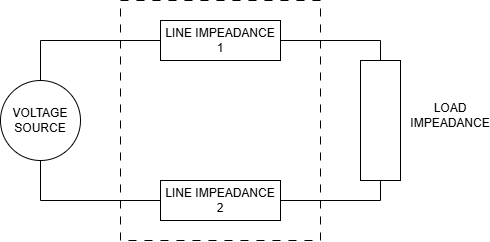
As engineers, we are almost always given the supply voltage. This is typically derived from the utility company. From our design and layout of the light poles, we can determine the Power demands of the load, which is simply the sum of all downstream lights (or other loads.) Using "Tribal knowledge" we can have a good idea of what size conductors we would need to use. We will pick one wire size and then calculate the voltage drop. Typically the voltage drop is 3% or less. If the voltage drop is higher, we will increase the wire size. Since we have the wire size, we can use the NEC Chapter 9 tables to determine the impeadance of the conductor, which also at this time factors in the power factor. Allow me to point as well that this closed circuit has the same current from the source, through each side of the line impeadance (explained in following paragraph) through the load, then to return to the source. To put another way, "I" is congruent through out and you'll see in my subscripts no indication from which place it belongs. So to summarize we have:

Consuetude: The First Order Equation

You may skip this section and go to "Inspection" if you are not intrested in the current NEC method.

This will describe briefly the current method and demonstrate where the logical fault is that I hope to emphasis here. I'll admit this is a quick summary just to get to the point. Firstly the issue is finding Voltage drop on the line. We shall start with these relationships and facts:

$$ V_{\text{line}} = V_{\text{SOURCE}} - V_{\text{load}} \tag{1} $$

$$ I_{\text{source}} = I_{\text{source}} = I_{\text{source}} \tag{2} $$

$$ V_{\text{line}} = I \cdot Z_{\text{LINE}} \tag{3} $$

$$ P_{\text{LOAD}} = V_{\text{source}} \cdot I \tag{4} $$

$$ I = \frac{P_{\text{LOAD}}}{V_{\text{SOURCE}}} \tag{5} $$

Now we can subsitute this value for current into our equation for voltage drop on the line to get:

$$ V_{\text{line}} = \frac{P_{\text{LOAD}}}{V_{\text{SOURCE}}} \cdot Z_{\text{LINE}} \tag{6} $$

This is a simple formula but again, THIS IS NOT CORRECT. The correct way to navigate this occuring issue where we need to find the loop current I is detailed below.

Inspection

Please note that for the sake of consistency and clarity, known quantities will have all capital subscript, unknown quantities will have lowercase subscript.

$$ P_{\text{LOAD}} = V_{\text{load}} \cdot I \tag{7} $$

$$ V_{\text{line}} = V_{\text{SOURCE}} - V_{\text{load}} \tag{8} $$

Equation 1 describes the power at the load end. Since PLOAD is known, the current through the system can be found. This is useful as we will use it to calculate the voltage drop on the line by simply using ohms's law. Equation 2 can be set up to solve for the voltage at the load, Vload. Then Ohm's law can be subsitute to write Vline (Voltage drop on the line) as an expression of current, and impeadance (which we know as well):

$$ V_{\text{load}} = V_{\text{SOURCE}} - V_{\text{line}} \tag{9} $$

$$ V_{\text{load}} = V_{\text{SOURCE}} - I \cdot Z_{\text{LINE}} \tag{10} $$

Now we can subsitute the expression for current from equation 1 into this equation to get an expression to relate PLOAD and I, in effort to achieve our goal of determining I:

$$ P_{\text{LOAD}} = (V_{\text{SOURCE}} - I \cdot Z_{\text{LINE}}) \cdot I \tag{11} $$

Manipuli Mathematica

Now we have an equation with only one unknown, I. We can solve for this, unfortunately using math.

We begin by distributing the current I term:

$$ P_{\text{LOAD}} = V_{\text{SOURCE}} \cdot I - Z_{\text{LINE}} \cdot I^2 \tag{12} $$

$$ V_{\text{SOURCE}} \cdot I - Z_{\text{LINE}} \cdot I^2 - P_{\text{LOAD}} = 0 \tag{13} $$

$$ Z_{\text{LINE}} \cdot I^2 - V_{\text{SOURCE}} \cdot I + P_{\text{LOAD}} = 0 \tag{14} $$

Now we have a quadratic equation in the form of

$$ ax^2 + bx + c = 0 \tag{15} $$

$$ I = \frac{-b \pm \sqrt{b^2 - 4ac}}{2a} \tag{16} $$

Substituting our values for a, b, and c we get:

$$ I = \frac{V_{\text{SOURCE}} \pm \sqrt{V_{\text{SOURCE}}^2 - 4Z_{\text{LINE}}P_{\text{LOAD}}}}{2Z_{\text{LINE}}} \tag{17} $$

Now we have an expression for the current I. We can then subsitute this back into our equation for voltage drop to get the voltage drop on the line. Notice the bottom term cancels:

$$ V_{\text{line}} = I \cdot Z_{\text{LINE}} \tag{18} $$

$$ V_{\text{line}} = \frac{V_{\text{SOURCE}} \pm \sqrt{V_{\text{SOURCE}}^2 - 4Z_{\text{LINE}}P_{\text{LOAD}}}}{2} \tag{19} $$

You may recall that the ZLINE term is derived from the NEC Chapter 9 tables based on the wire size and power factor. This is for only one conductor going one direction. The reason for doing this is that in 3 Phase there is multiple conductors. Thus the voltage drop VLINE is actually the Vline from our equation simply multiplied by 2 for the 2 separate runs of conductors. This simplifieds our equation even more:

$$ V_{\text{line}} = V_{\text{SOURCE}} \pm \sqrt{V_{\text{SOURCE}}^2 - 4Z_{\text{LINE}}P_{\text{LOAD}}} \tag{20} $$

If we take only the subtraction of the square root, we get an equation similar to our orignal equation 2. Equation 2 has been included for comparison:

$$ V_{\text{line}} = V_{\text{SOURCE}} - \sqrt{V_{\text{SOURCE}}^2 - 4Z_{\text{LINE}}P_{\text{LOAD}}} \tag{21} $$

$$ V_{\text{line}} = V_{\text{SOURCE}} - V_{\text{load}} \tag{22} $$

It should now be obvious as well that the voltage on the load, Vload, can be expressed as:

$$ V_{\text{load}} = \sqrt{V_{\text{SOURCE}}^2 - 4Z_{\text{LINE}}P_{\text{LOAD}}} \tag{23} $$

Conclusions of the Quadratic kind

Now we have an accurate equation for the voltage drop on the line. We can then calculate the percentage voltage drop by dividing this by the source voltage. If this is above 3%, we would need to increase the wire size and recalculate. This process is repeated until we get a voltage drop of 3% or less. Here is a conclusion of the useful equations derived from the quadratic formula manipulation:

$$ I = \frac{V_{\text{SOURCE}} \pm \sqrt{V_{\text{SOURCE}}^2 - 4Z_{\text{LINE}}P_{\text{LOAD}}}}{2Z_{\text{LINE}}} \tag{24} $$

$$ V_{\text{line}} = V_{\text{SOURCE}} - \sqrt{V_{\text{SOURCE}}^2 - 4Z_{\text{LINE}}P_{\text{LOAD}}} \tag{25} $$

$$ V_{\text{load}} = \sqrt{V_{\text{SOURCE}}^2 - 4Z_{\text{LINE}}P_{\text{LOAD}}} \tag{26} $$

Here is the expression, simplified, for the percentage voltage drop:

$$ \text{Total Line Voltage Drop Percentage} = \frac{V_{\text{line}}}{V_{\text{SOURCE}}} = 1 - \sqrt{1 - \frac{4Z_{\text{LINE}}P_{\text{LOAD}}}{V_{\text{SOURCE}}^2}} \tag{27}$$

These equations, to be continued, expanded, and berated in a different chapter, can be utilized in either an iterative fashion or with a matrix for the rapid calculation and optomization of running large arrays of branches and loads. This is common in lighting design for large parking lots, stadiums, and other large outdoor areas. The lights are not necessarily evenly distributed from a circuit perspective, so careful calculation is required. They are not simply combined in a lattice chain (unless they are.) The goal is to minimize the voltage drop while also minimizing the cost of the project, which is typically dominated by the cost of the conductors. By these means we have completely characterized an analysis of a single branch lighting circuit.

fin